Bilbao Crystallographic Server Subperdiodic Groups Help SECTIONS

Basic concepts

SECTIONS determines the layer symmetry of plane sections obtained by intersecting a crystal structure with space-group symmetry \mathcal{G} with a family of rational (diperiodic) planes. This family is defined by the normal vector \bm{n}^{*}=h\bm{a}^{*}+k\bm{b}^{*}+\ell\bm{c}^{*}, specified by the integer Miller indices (hk\ell) in the reciprocal basis (\bm{a}^{*},\ \bm{b}^{*},\ \bm{c}^{*}) associated to the basis (\bm{a},\ \bm{b},\ \bm{c}) of \mathcal{G}.
As input only \mathcal{G} and \bm{n}^{*} are needed. The space group to scan, \mathcal{G}, can be input by its number given in the International Tables for Crystallography Vol. A (ITA) or by a set of generators in the form of (x,y,z) triplets. These triplets are also in ITA for all the standard settings of the space groups. The symmetry operations of \mathcal{G} can be expressed in any basis useful to the user, through either a transformation matrix (see the Appendix for some common and useful transformations) when the standard number of \mathcal{G} is supplied, or by a set of generators given in the basis chosen by the user and supplied also as (x,y,z) triplets. Note that the scanned object is periodic, and therefore the solution will also be periodic.

With these data the program basically perform the following actions:

1. First the direction of periodicity of the section crystal pattern is determined. This is the so-called scanning vector \bm{d}. In many occasions \bm{d} is parallel to \bm{n}^{*} and therefore, it is a translation of \mathcal{G} perpendicular to the plane sections. However, this is not general and depends on the layer symmetry. When this choice for \bm{d} is not possible, the scanning vector is determined by a translation (the solution is not unique) with the shortest projection on \bm{n}^{*}. Each section is positioned along \bm{d} by its distance s to the origin of \mathcal{G}.
2. Then the interesting values of s (or levels along the scanning vector) are calculated. s can have special values with fixed numerical values and/or general values referred simply by s, which are arbitrary but different from the special values. Given the periodicity of the solution, s is considered to be in the interval [0,1).
3. Finally, the layer symmetry of each section at s\bm{d} is calculated.

The program returns \bm{d}, the analyzed values of s and the layer groups corresponding to each particular plane section. The layer groups appear in their standard settings, given in the Vol. E of the International Tables for Crystallography (ITE). The conventional bases of the layer groups are also expressed in terms of the basis chosen for the space group \mathcal{G}.

To understand the above concepts of space group scanning, consider the scanning of the space group P622 (No. 177) in its standard setting, through (001) plane sections. Figure 1a) shows the diagram of the symmetry elements of this space group as given in ITA. The normal to the (001) planes \bm{c}^{*}, is perpendicular to the plane of projection and coincides in direction with \bm{c}, which is the scanning vector \bm{d}. The distribution of symmetry elements is repeated periodically for planes at the special values \frac{1}{2}\bm{c}, \bm{c}, \cdots and keep the plane sections at z=s=0,\ \frac{1}{2},\ ,1,\dots invariant. The layer symmetry of these planes is p622 (No. 76). For any other value of z=s, i.e. for general values of s, the twofold and twofold screw axes lying on the special sections z=0,\ \frac{1}{2},\ 1, etc. are lost [see Figure 1b)] and the symmetry of the corresponding plane sections is reduced to the layer group p6. (No. 73)

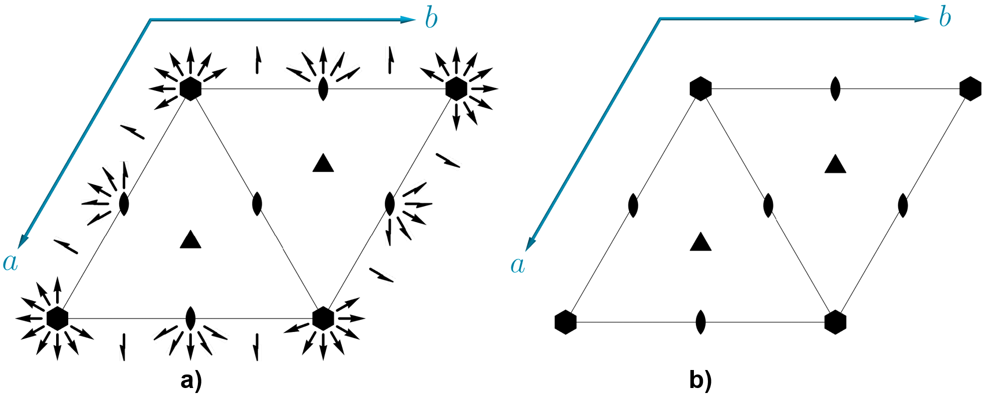Fig 1. a) Diagram for the symmetry elements of the space group \mathcal{G}=P622 (No. 177). Note that periodicity along \bm{c} generates new symmetry operations that are equally distributed at \ \frac{1}{2},\ ,1,\dots and keep the corresponding plane sections at those special z-values (or equivalently s-values), invariant. The corresponding layer group is p622 (No. 76). b) Symmetry elements of the space group p622 present at an arbitrary value of z. For a section at these z (or s), the layer group is p6 (No. 73).

Use of the program

Now we can analize this simple problem with the program SECTIONS. The required input consists of the space-group number, specified on the previous page (not shown), and the Miller indices of the normal vector:

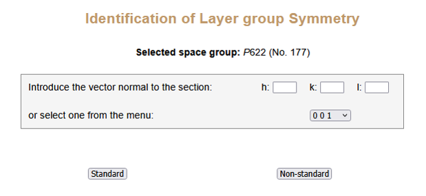
In this case the normal vector has been selected from the drop-down menu. The button Non-standard allows the introduction of a transformation matrix, not used in this example. After clicking on the Standard button, the output appears:

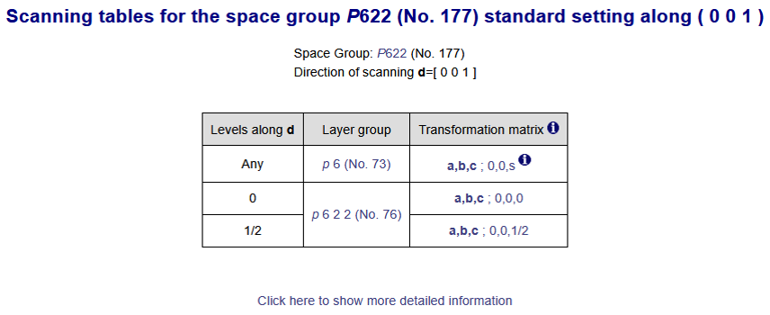
The scanning vector is \bm{d}=[0 0 1], the lattice vector \bm{c} of the input basis. Then, a table with three columns, summarizes this scanning. The first column indicates the distances s along \bm{d} from the origin of the space group to the intersections of the plane sections with \bm{d}. The second column contains the standard symbol and number of the layer group of each plane section. The third column gives the transformation matrix that relates the standard basis of the layer group with the basis of the input space group (\bm{a},\bm{b},\bm{c}), whether or not it is standard. The origin shift with respect to the origin of the scanned space group is given after a semicolon.

Any means a variable value of s, in the interval s \in [0,1), excluding the fixed values of s given below. The layer symmetry of these planes is always a polar layer group, in this case p6. The standard basis is the input basis and the standard origins of the scanned space group and the sectional layer group, coincide. The sections with fixed parameters s=0 and s=\frac{1}{2} share the same sectional layer group p622 with the same basis vectors on the plane sections. The origin shift of the plane section at s=\frac{1}{2} reflects the position of the section with respect to the origin of the space group.

Clicking over a layer group, will show its symmetry operations in the standard setting. Clicking on a transformation matrix will list paired, the symmetry operations of the layer group in its standard setting and in the basis of the scanned space group. For the latter, the lattice translations are not reduced to the interval [0,1) to show which symmetry operations of the space group are part of the layer group. Below the table is a link that provides access to more detailed information about the scan. This is described in the following section.

More detailed information: the scanning group and linear orbits

After clicking on the link to request more detailed information, the full output of the program is:

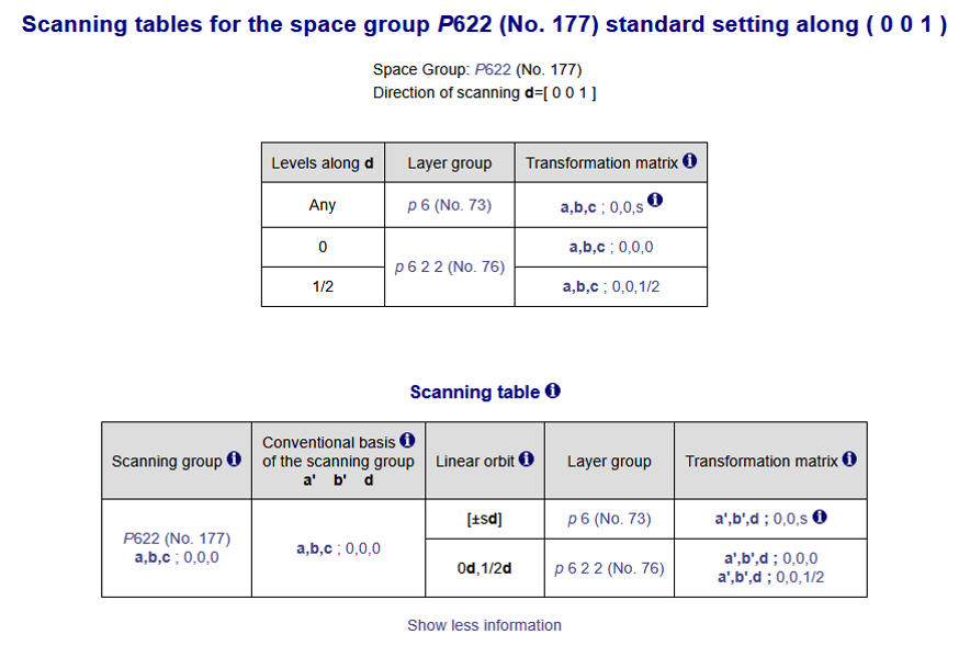
The scanning table includes information about the so-called scanning group and linear orbits.

The scanning group \mathcal{H}, is a subgroup of the scanned space group \mathcal{G}, that includes all the symmetry operations \{R|\bm{t}\} of \mathcal{G} that invert or keep invariant \bm{n}^{*}: \mathcal{H}=\left\{\{R|\bm{t}\} \in \mathcal{G}|\bm{n}^{*}R^{-1}=\pm\bm{n}^{*}\right\}

Since the translations of \mathcal{G}, \{E|\bm{T}\}, fulfill such condition, the scannig group \mathcal{H} is a translationengleiche subgroup of \mathcal{G}. It appears in the first column together with a transformation matrix that expresses its standard (default choice) ITA basis in terms of the user basis.

The second column shows a conventional (symmetry-adapted) basis for \mathcal{H}, denoted by (\bm{a}',\bm{b}',\bm{d}), such that \bm{a}' and \bm{b}' lie on the plane section and \bm{d} is the scanning direction.

The last column labeled transformation matrix gives the standard bases of the sectional layer groups as linear combinations of the conventional basis (\bm{a}',\bm{b}',\bm{d}) of the scanning group.

The third column shows the (linear orbits), the set of parallel plane sections that share the same layer symmetry. The linear orbits are generated by the application of the symmetry operations of \mathcal{H} (not included in the sectional layer groups of the section) on a certain plane section.

Continuing with the case at hand, the scanning table shows the following linear orbits:

1. [\pm s\bm{d}]. This case corresponds to planes at arbitrary position s\bm{d}. The sectional layer group for these family of planes is p6. It means that the twofold axes through the origin of \mathcal{H}, that in this case is equal to \mathcal{G}, [see Figure 1a)], transforms the plane at s\bm{d} into a plane at -s\bm{d} with the same layer symmetry. Therefore, both planes belong to the same linear orbit and both positions are enclosed by brackets. [\pm s\bm{d}] is a compact form of [s\bm{d}, 1-s\bm{d}] if we want to restrict s within the interval [0,1).
2. 0\bm{d} and \frac{1}{2}\bm{d}. In these cases the layer symmetry is p622, so there are no more symmetry operations in \mathcal{H}. Therefore the plane sections although sharing the same layer group, they not belong to the same orbit. In that cases the notation includes both positions but without brackets surrounding them.

The notation for orbits shown in SECTIONS, follows that used in ITE where all possible cases are analized.

Appendix

Some transformation matrices and origin shifts

Useful three-dimensional transformation matrices (\mathbf{P} and \mathbf{Q}=\mathbf{P}^{-1}) extracted from the International Tables for Crystallography Vol. A, where the full list (see there the table 1.5.1.1) of the most relevant transformation matrices are given. \begin{array}{lll} \qquad\qquad\qquad\text{\textbf{Transformation}}&\qquad\quad\mathbf{P}&\quad\ \mathbf{Q}=\mathbf{P}^{-1}\\[2pt] \hline\\ \text{Unique axis } \mathbf{b} &&\\ \text{Cell choice 1}\rightarrow \text{Cell choice 2:} \left\{ \begin{array}{l} P\ \rightarrow \ P \\ C\ \rightarrow \ A \end{array} \right. & &\\[5mm] \text{Cell choice 2}\rightarrow \text{Cell choice 3:} \left\{ \begin{array}{l} P\ \rightarrow \ P \\ A\ \rightarrow \ I \end{array} \right. & \left( \begin{array}{ccc} \bar{1}&0&1 \\ 0&1&0 \\ \bar{1}&0&0 \end{array}\right) & \left( \begin{array}{ccc}0&0&\bar{1} \\ 0&1&0 \\ 1&0&\bar{1} \end{array}\right)\\[5mm] \text{Cell choice 3}\rightarrow \text{Cell choice 1:} \left\{ \begin{array}{l} P\ \rightarrow \ P \\ I\ \ \rightarrow \ C \end{array} \right. & &\\[3mm] % \hline\\ \text{Unique axis } \mathbf{c} & & \\ \text{Cell choice 1} \rightarrow \text{Cell choice 2:} \left\{ \begin{array}{l} P\ \rightarrow \ P \\ A\ \rightarrow \ B \end{array} \right. & &\\ \text{Cell choice 2} \rightarrow \text{Cell choice 3:} \left\{ \begin{array}{l} P\ \rightarrow \ P \\ B\ \rightarrow \ I \end{array} \right. & \left( \begin{array}{ccc} 0&\bar{1}&0 \\ 1&\bar{1}&0 \\ 0&0&1 \end{array}\right) & \left( \begin{array}{ccc} \bar{1}&1&0 \\ \bar{1}&0&0 \\ 0&0&1 \end{array}\right)\\ \text{Cell choice 3} \rightarrow \text{Cell choice 1:} \left\{ \begin{array}{l} P\ \rightarrow \ P \\ I\ \ \rightarrow \ A \end{array} \right. & &\\[3mm] % \hline\\ \text{Unique axis } \mathbf{b} \ \rightarrow \ \text{unique axis } \mathbf{c} & \\[2mm] \text{Cell choice 1:} \left\{ \begin{array}{l} P\ \rightarrow \ P \\ C\ \rightarrow \ A \end{array} \right. & &\\ \text{Cell choice 2:} \left\{ \begin{array}{l} P\ \rightarrow \ P \\ A\ \rightarrow \ B \end{array} \right. & \left( \begin{array}{ccc} 0&1&0 \\ 0&0&1 \\ 1&0&0 \end{array}\right) & \left( \begin{array}{ccc} 0&0&1 \\ 1&0&0 \\ 0&1&0 \end{array}\right)\\ \text{Cell choice 3:} \left\{ \begin{array}{l} P\ \rightarrow \ P \\ I\ \ \rightarrow \ I \end{array} \right. & &\\[3mm] \hline\\ \text{Primitive rhombohedral cell} \rightarrow \text{hexagonal cell R, obverse setting} & \left( \begin{array}{ccc} 1&0&1 \\ \bar{1}&1&1 \\ 0&\bar{1}&1 \end{array}\right) & \left( \begin{array}{ccc} \frac{2}{3}&\frac{\bar1}{3}&\frac{\bar{1}}{3} \\[0.5mm] \frac{1}{3}&\frac{1}{3}&\frac{\bar{2}}{3} \\[0.5mm] \frac{1}{3}&\frac{1}{3}&\frac{1}{3} \end{array}\right)\\[6.5mm] \hline % \end{array}

Origin shifts, given as transformation matrices, relating the origin choice 1 to the origin choice 2. Use them in SECTIONS to get the results in the origin choice 1 description of the following space groups: \begin{array}{l|c} \qquad\qquad\qquad\qquad\qquad\qquad\qquad\text{\textbf{Space groups}}&\text{\textbf{Origin shift}}\\[1mm] \hline\\[-3mm] Pnnn\text{ (No. \textbf{48})} & \bm{a},\bm{b},\bm{c};\frac{1}{4},\frac{1}{4},\frac{1}{4}\\[1mm] Pban\text{ (No. \textbf{50}), } Pmmn\text{ (No. \textbf{59})} & \bm{a},\bm{b},\bm{c};\frac{1}{4},\frac{1}{4},0\\[1mm] Ccce\text{ (No. \textbf{68})} & \bm{a},\bm{b},\bm{c};0,\frac{1}{4},\frac{1}{4}\\[1mm] Fddd\text{ (No. \textbf{70}), } Fd\bar{3}\text{ (No. \textbf{203}), } Fd\bar{3}m\text{ (No. \textbf{227})}& \bm{a},\bm{b},\bm{c};\bar{\frac{1}{8}},\bar{\frac{1}{8}},\bar{\frac{1}{8}}\\[1mm] P4/n\text{ (No. \textbf{85}), } P4/nmm\text{ (No. \textbf{129}), } P4/ncc\text{ (No. \textbf{130})}& \bm{a},\bm{b},\bm{c};\bar{\frac{1}{4}},\frac{1}{4},0\\[1mm] P4_{2}/n\text{ (No. \textbf{86}), } P4/nnc\text{ (No. \textbf{126}), } Pn\bar{3}\text{ (No. \textbf{201}), } Pn\bar{3}n\text{ (No. \textbf{222}), } Pn\bar{3}m\text{ (No. \textbf{224})}& \bm{a},\bm{b},\bm{c};\bar{\frac{1}{4}},\bar{\frac{1}{4}},\bar{\frac{1}{4}}\\[1mm] I41_{1}/a \text{ (No. \textbf{88})}& \bm{a},\bm{b},\bm{c};0,\bar{\frac{1}{4}},\bar{\frac{1}{8}}\\[1mm] P4/nbm\text{ (No. \textbf{125})} & \bm{a},\bm{b},\bm{c};\bar{\frac{1}{4}},\bar{\frac{1}{4}},0\\[1mm] P4_{2}nbc\text{ (No. \textbf{133}), } P4_{2}/nnm\text{ (No. \textbf{134}), } P4_{2}/nmc\text{ (No. \textbf{137}), } P4_{2}/ncm\text{ (No. \textbf{138})}& \bm{a},\bm{b},\bm{c};\bar{\frac{1}{4}},\frac{1}{4},\bar{\frac{1}{4}}\\[1mm] I4_{1}/amd\text{ (No. \textbf{141}), } I4_{1}/acd\text{ (No. \textbf{142})}& \bm{a},\bm{b},\bm{c};0,\frac{1}{4},\bar{\frac{1}{8}}\\[1mm] Fd\bar{3}c\text{ (No. \textbf{228})} & \bm{a},\bm{b},\bm{c};\bar{\frac{3}{8}},\bar{\frac{3}{8}},\bar{\frac{3}{8}}\\[1mm] \hline \end{array}

References

1. V. Kopský, Ferroelectrics 111, 1, 81-85 (1990). The scanning group and the scanning theorem for layer and rod groups.

2. International Tables for Crystallography Vol. A: Space-group symmetry (2016). (Edited by M.I. Aroyo): H. Wondratscheck and M.I. Aroyo, Origin shift and change of the basis. Chapter 1.5, pp. 75-83.